 Gather
Gather function takes multiple table columns and collapses into key-value pairs, duplicating all other columns as needed.
Properties
| Variables to Gather |
Using this property, we define the variables (columns) that we want to transform into rows. |
| Key |
The name of the new variable (column), which will contain the names of gathered columns. |
| Value |
The name of a new variable (column) that will contain values from the gathered columns. |
| Remove Empty |
Boolean. Property defines whether the row will be deleted if it contains an blank cell in the Value variable. |
Keywords
Columns to Rows, Unpivot Pivot Excel Table, Unpivot Table, Data Unpivoting, Wide Form Table to Long
See Also
Transpose,
Spread,
Flip_Vertical,
Flip_Horizontal
Video-tutorial
How to Unpivot Excel Data
It is often the case that we get the data from a customer or colleagues in the “Wide Form” format. An example may be some summary statistic for several categories that are stored side by side in the columns. For further work, however, we need these data not in columns but in rows. This transformation is also called as Unpivoting. With the Reshape.XL add-in, you can do this using the Gather function. An example of its use is in the following illustration.
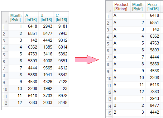
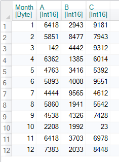
As an example, we use the following table, where we have the amount of products sales (A,B and C) in each month. Our task is to transform this table so we get a new table with three columns. In the first column will be stored Product ID (A, B or C), in the second will be integer Month values (1 to 12) and in the third will be sales values (Price).
For this data transformation click the Gather button in the ribbon toolbar tab Reshape.

If you click on the added function in the sidebar, its properties will appear in the Properties Panel. These settings are divided into two tabs - Basic Properties and Other. In the first panel, you can select from the list of variables the ones you want to transform - unpivot.
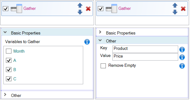
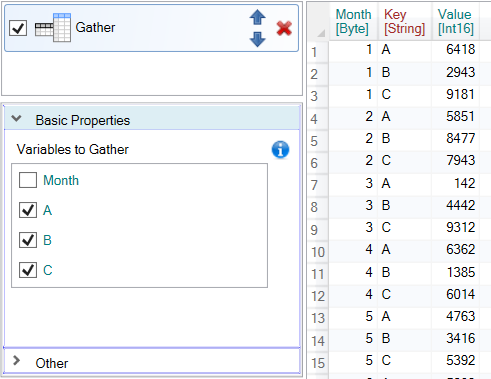
In the example we selected the variables A, B and C. The result of this setting is shown in the following figure. As a result, we created three variables - Month, Key (Product ID) and Value (sum of sales).
Under the Other tab, you find additional auxiliary settings. Using the properties Key and Value, you can define the names of newly created columns. In the following example, we changed the column names to Product and Price.
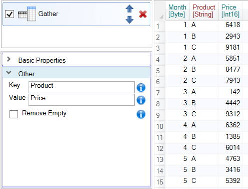
In addition to the described properties here stayed one more - Remove Empty. Using this property you can decide whether a new record will be created if the cell from the input table is empty. If you set the property to TRUE, the empty cells will be ignored.
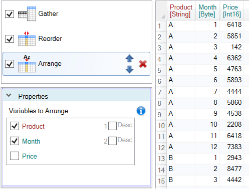
After data unpivoting, it may be necessary to modify the resulting table. In the last example, we used the Reorder function to change the order of individual columns in the table and Arrange to sort the records. The individual records were sorted by Product and Month variables.
If you want to apply the opposite process to your data - Pivoting - to create several new columns from the Key - Value variable pair (rows to columns), use the Spread function.